Network meta-analysis in R

Meta-analysis (MA) has gained more popularity in Plant Pathology. Among the methods, network meta-analysis has been thoroughly presented to plant pathologists in a recent paper. In this post, I reproduce part of the analysis shown in that paper which was conducted using SAS. Although the results are not identical, they are very similar.

Why and who is this post for?

Meta-analysis (MA) has gained popularity in plant pathology. Among the several meta-analytic methods, Network Meta-Analysis (NMA) models, also known as Mixed Treatment Comparison (MTC), has been thoroughly presented to plant pathologists in a recent review paper published in Phytopathology® Madden et al. (2016).

Results of a recent survey (Del Ponte, unpublished) showed that more than 50 meta-analysis articles have been published using plant disease-related data, mainly to test treatment effects on disease severity and yield, but also their relationship, among other effects of interest. Although this is a VERY small number of studies compared with other fields (medicine and psychology), a trend towards increasing its use in our field is evident.

Specifically, multiple treatment comparison (e.g., fungicides and biocontrol agents) is usually of interest and these treatments are usually compared with a common treatment, the untreated check, with their effects (relative control) thus being correlated. Hence, this post is for those interest in learning how to fit network meta-analysis models, in particular the frequentist and arm-based approach (as opposed to contrast-based) using open source tools, as alternative to SAS and other commercial software.

Here, I reproduce the analysis shown in a paper where the authors made available all the data (wheat yield response to fungicides), as well as SAS codes Madden et al. (2016), using an MA-specific package of R, {metafor}. Here I fitted the same model, the arm-based or unconditional, similar to the original paper. In that case, his approach the effect sizes are directly the treatment means and not the difference or ratio as traditionally performed in meta-analysis).

I will reproduce some, not all, of the arm-based models presented in the original paper using {metafor}. I will explain most of the important details about how to prepare the data, visualize the responses, fit the models and compare results with the original paper. Anyone should be able to reproduce the analysis below by copying and pasting into R. To facilitate instant access and reproducibility, I created an RStudio project in the cloud where anyone can run this code and get the same results. Click here to get access to the RStudio project in the cloud.

Data preparation

The data were obtained from the supplemental FileS1, a SAS file that contains the documented code and the data. Here, the data were organized in one MS Excel file following the same original structure and content, excepting that missing data was represented by an empty cell. Let’s load some packages for data importing and wrangling.

library(tidyverse) # load several useful pkgs
library(readxl) # import excel data

Now we are ready to import the data and convert both yield and variance to metric unit as performed in the paper. Note: we do not need to create the weight variable as in the SAS code because this is handled in the meta-analysis specific R packages.

wheat0 <- read_excel("wheat.xlsx")
wheat <- wheat0 %>%
  mutate(varyld = (1 / wtyield) * (0.0628 ^ 2),
         yield = yield * 0.0628) %>%
  na.omit() # here we omit the rows with missing data

Let’s replace the names of the levels of the treatment factor from numbers to the fungicide treatment acronym.

wheat <- wheat %>%
  mutate(trt = replace(trt, trt == 10, "CTRL")) %>%
  mutate(trt = replace(trt, trt == 2, "TEBU")) %>%
  mutate(trt = replace(trt, trt == 3, "PROP")) %>%
  mutate(trt = replace(trt, trt == 4, "PROT")) %>%
  mutate(trt = replace(trt, trt == 5, "TEBU+PROT")) %>%
  mutate(trt = replace(trt, trt == 6, "MET"))

Meta-analytic (arm-based) model

I use here the {metafor} package, a free and open-source add-on for conducting meta-analyses with the statistical software environment R. I followed the example for fitting the arm-based network MA as shown in this presentation and this documentation by the author of the package.

In the original NMA paper, the authors compared three different variance-covariance matrix for a random-effects model: compound symmetry (CS), heterogeneous CS (HCS) and unstructured (UN). These can be informed directly in the rma.mv() function. OK, let’s load {metafor} package now.

library(metafor)

Now we can fit the first model, model R1 in the paper, with compound symmetry (CS) structure for the variance-covariance matrix Madden et al. (2016). This is used because all treatments within a study share the same random effect, all treatments are correlated, with a covariance for pairs of treatments given by the between-study variance Madden et al. (2016).

We use the rma.mv() function that allows fitting mixed effects model for multivariate and multi-treatment situations. The first two arguments are the effect of interest, which is yield (means of the treatment of interest across replicates within the same trial) and the sampling variance varyld (e.g., the residual variance obtained from the fit of an ANOVA like model). Our moderators is the factor of interest, in our case treatment trt. The method is the maximum likelihood. The random component will be treatment and trial, meaning a random intercept for treatments within trials, which are also random. The struct is CS and the data is wheat.

net_arm_CS <- rma.mv(
  yield,
  varyld,
  mods = ~ trt,
  method = "ML",
  random = list( ~ trt | factor(trial)),
  struct = "CS",
  data = wheat
)

We call the summary results of the model. Let’s jump straight to model results where we can check the estimates for each treatment which are the differences to the intercept, defined as the untreated check. We can see that MET (0.436 ton) and PROP (0.20 ton) provided the highest and lowest numerical yield difference relative to the untreated (intercept). We should also look at the 95% confidence intervals.

summary(net_arm_CS)

Multivariate Meta-Analysis Model (k = 558; method: ML)

   logLik   Deviance        AIC        BIC       AICc   
-283.5052  1710.1250   583.0105   617.6054   583.2728   

Variance Components:

outer factor: factor(trial) (nlvls = 136)
inner factor: trt           (nlvls = 6)

            estim    sqrt  fixed 
tau^2      1.5516  1.2456     no 
rho        0.9841             no 

Test for Residual Heterogeneity:
QE(df = 552) = 55024.7841, p-val < .0001

Test of Moderators (coefficients 2:6):
QM(df = 5) = 319.9986, p-val < .0001

Model Results:

              estimate      se     zval    pval   ci.lb   ci.ub      
intrcpt         3.5335  0.1076  32.8500  <.0001  3.3227  3.7443  *** 
trtMET          0.4360  0.0309  14.1295  <.0001  0.3755  0.4965  *** 
trtPROP         0.1994  0.0361   5.5206  <.0001  0.1286  0.2702  *** 
trtPROT         0.4286  0.0365  11.7560  <.0001  0.3572  0.5001  *** 
trtTEBU         0.2744  0.0258  10.6558  <.0001  0.2239  0.3249  *** 
trtTEBU+PROT    0.4326  0.0306  14.1523  <.0001  0.3727  0.4925  *** 

---
Signif. codes:  0 '***' 0.001 '**' 0.01 '*' 0.05 '.' 0.1 ' ' 1

Heterogeneous CS

Alternatively, between-study variance can be considered unequal when there is an overall random study effect. In this model, there is a constant between-study correlation for all pairs of treatments with unequal between-study total variances, and this matrix is called heterogeneous compound symmetry (HCS). This the R2 model in Madden et al. (2016).

# Be patient. The model fit may take more than a minute to finish running
net_arm_HCS <- rma.mv(
  yield,
  varyld,
  mods = ~ trt,
  method = "ML",
  random = list( ~ trt | factor(trial)),
  struct = "HCS",
  data = wheat
)

Compare the results with the previous model.

summary(net_arm_HCS)

Multivariate Meta-Analysis Model (k = 558; method: ML)

   logLik   Deviance        AIC        BIC       AICc   
-278.3457  1699.8060   582.6915   638.9082   583.3606   

Variance Components:

outer factor: factor(trial) (nlvls = 136)
inner factor: trt           (nlvls = 6)

            estim    sqrt  k.lvl  fixed      level 
tau^2.1    1.6636  1.2898    136     no       CTRL 
tau^2.2    1.4271  1.1946     86     no        MET 
tau^2.3    1.5232  1.2342     57     no       PROP 
tau^2.4    1.5315  1.2375     56     no       PROT 
tau^2.5    1.5312  1.2374    136     no       TEBU 
tau^2.6    1.5056  1.2270     87     no  TEBU+PROT 
rho        0.9848                    no            

Test for Residual Heterogeneity:
QE(df = 552) = 55024.7841, p-val < .0001

Test of Moderators (coefficients 2:6):
QM(df = 5) = 301.4403, p-val < .0001

Model Results:

              estimate      se     zval    pval   ci.lb   ci.ub      
intrcpt         3.5379  0.1113  31.7790  <.0001  3.3197  3.7561  *** 
trtMET          0.4334  0.0312  13.8703  <.0001  0.3722  0.4947  *** 
trtPROP         0.1946  0.0360   5.4039  <.0001  0.1240  0.2651  *** 
trtPROT         0.4263  0.0364  11.7284  <.0001  0.3551  0.4976  *** 
trtTEBU         0.2687  0.0260  10.3307  <.0001  0.2177  0.3196  *** 
trtTEBU+PROT    0.4290  0.0307  13.9841  <.0001  0.3688  0.4891  *** 

---
Signif. codes:  0 '***' 0.001 '**' 0.01 '*' 0.05 '.' 0.1 ' ' 1

Unstructured matrix

Finally, we fit now the model with an unstructured (UN) variance-covariance matrix. Here, we allow the matrix to be completely unstructured, with different variance for each treatment or different covariance (correlation) for each pair of treatments. Note: I needed to use an optimizer (see the control argument) for convergence.

# Be more patient. This may take much longer to complete run.
net_arm_UN <- rma.mv(
  yield,
  varyld,
  mods = ~ trt,
  method = "ML",
  random = list( ~ trt | factor(trial)),
  struct = "UN",
  control = list(optimizer = "nlm"),
  data = wheat
)

We can then check results:

summary(net_arm_UN)

Multivariate Meta-Analysis Model (k = 558; method: ML)

    logLik    Deviance         AIC         BIC        AICc   
-2161.8323   5466.7791   4377.6646   4494.4223   4380.5175   

Variance Components:

outer factor: factor(trial) (nlvls = 136)
inner factor: trt           (nlvls = 6)

               estim     sqrt  k.lvl  fixed      level 
tau^2.1    2026.0759  45.0120    136     no       CTRL 
tau^2.2    1078.5412  32.8412     86     no        MET 
tau^2.3     557.8729  23.6193     57     no       PROP 
tau^2.4     453.8729  21.3043     56     no       PROT 
tau^2.5    2443.9082  49.4359    136     no       TEBU 
tau^2.6     492.9330  22.2021     87     no  TEBU+PROT 

           rho.CTRL  rho.MET  rho.PROP  rho.PROT  rho.TEBU  rho.TEBU+ 
CTRL              1                                                   
MET          0.9193        1                                          
PROP         0.8580   0.9357         1                                
PROT         0.8221   0.8897    0.9125         1                      
TEBU         0.8060   0.8674    0.9056    0.9411         1            
TEBU+PROT    0.4117   0.5540    0.5471    0.5945    0.5635          1 
             CTRL  MET  PROP  PROT  TEBU  TEBU+ 
CTRL            -   86    57    56   136     87 
MET            no    -    42    41    86     74 
PROP           no   no     -    24    57     39 
PROT           no   no    no     -    56     47 
TEBU           no   no    no    no     -     87 
TEBU+PROT      no   no    no    no    no      - 

Test for Residual Heterogeneity:
QE(df = 552) = 55024.7841, p-val < .0001

Test of Moderators (coefficients 2:6):
QM(df = 5) = 0.1049, p-val = 0.9998

Model Results:

              estimate      se    zval    pval    ci.lb    ci.ub    
intrcpt         3.5388  3.8598  0.9168  0.3592  -4.0262  11.1038    
trtMET          0.4397  1.8054  0.2435  0.8076  -3.0989   3.9782    
trtPROP         0.2620  2.4810  0.1056  0.9159  -4.6008   5.1247    
trtPROT         0.4974  2.6605  0.1870  0.8517  -4.7171   5.7120    
trtTEBU         0.2661  2.5482  0.1044  0.9168  -4.7282   5.2605    
trtTEBU+PROT    0.5101  3.7118  0.1374  0.8907  -6.7648   7.7850    

---
Signif. codes:  0 '***' 0.001 '**' 0.01 '*' 0.05 '.' 0.1 ' ' 1

Model comparison

To facilitate comparison, we can extract the mean estimate and the respective standard error from each of the models namely R1 (CS), R2(HCS) and R3(UN) as in the original paper.

library(broom) # load this to use the tidy function

R1_mean <- tidy(round(net_arm_CS$b, 3))
R2_mean <- tidy(round(net_arm_HCS$b, 3))
R3_mean <- tidy(round(net_arm_UN$b, 3))
R1_se <- tidy(round(net_arm_CS$se, 3))
R2_se <- tidy(round(net_arm_HCS$se, 3))
R3_se <- tidy(round(net_arm_UN$se, 3))

And now we prepare a table for displaying the statistics and can compare with the original paper. We can notice that the results are very similar, although not identical.

table1 <-
  data.frame(R1_mean, R1_se, R2_mean, R2_se, R3_mean, R3_se)
colnames(table1) <-
  c("R1_mean", "R1_se", "R2_mean", "R2_se", "R3_mean", "R3_se")
table1$Treat <-
  c("CTRL", "MET", "PROP", "PROT", "TEBU", "TEBU+PROT")
knitr::kable(table1)

R1_mean	R1_se	R2_mean	R2_se	R3_mean	R3_se	Treat
3.534	0.108	3.538	0.111	3.539	3.860	CTRL
0.436	0.031	0.433	0.031	0.440	1.805	MET
0.199	0.036	0.195	0.036	0.262	2.481	PROP
0.429	0.036	0.426	0.036	0.497	2.661	PROT
0.274	0.026	0.269	0.026	0.266	2.548	TEBU
0.433	0.031	0.429	0.031	0.510	3.712	TEBU+PROT

Source of the figure

As in the original paper, we will compare all three models based on the LRT test (using the anova() function). The full model uses the UN variance-covariance matrix. Agreeing with the original study, the UN provided a better fit to the data based on the lowest AIC.

anova(net_arm_HCS, net_arm_CS)

        df      AIC      BIC     AICc    logLik     LRT   pval 
Full    13 582.6915 638.9082 583.3606 -278.3457                
Reduced  8 583.0105 617.6054 583.2728 -283.5052 10.3190 0.0667 
                QE 
Full    55024.7841 
Reduced 55024.7841 

anova(net_arm_CS, net_arm_UN)

        df       AIC       BIC      AICc     logLik    LRT   pval 
Full    27 4377.6646 4494.4223 4380.5175 -2161.8323               
Reduced  8  583.0105  617.6054  583.2728  -283.5052 0.0000 1.0000 
                QE 
Full    55024.7841 
Reduced 55024.7841 

anova(net_arm_HCS, net_arm_UN)

        df       AIC       BIC      AICc     logLik    LRT   pval 
Full    27 4377.6646 4494.4223 4380.5175 -2161.8323               
Reduced 13  582.6915  638.9082  583.3606  -278.3457 0.0000 1.0000 
                QE 
Full    55024.7841 
Reduced 55024.7841 

Forest plot

With the results in hand, a dot and error plot with treatments ordered from highest to lowest yield difference is a nice way to visualize the results - not identical but similar to a traditional forest plots. For such, we make the size of the dots proportional to the inverse of the standard error.

table1 %>%
  filter(Treat != "CTRL") %>%
  ggplot(aes(reorder(Treat, R3_mean), R3_mean)) +
  geom_point(aes(size = 1 / R3_se), shape = 15) +
  geom_errorbar(aes(ymin = R3_mean - R3_se,
                    ymax = R3_mean + R3_se), width = 0.01) +
  ylim(0.1, 0.6) +
  labs(
    y = "Yield difference (ton/ha)",
    x = "",
    title = "Yield response to fungicides",
    caption = "Data source: Madden et al. (2016)"
  ) +
  theme_light() +
  coord_flip()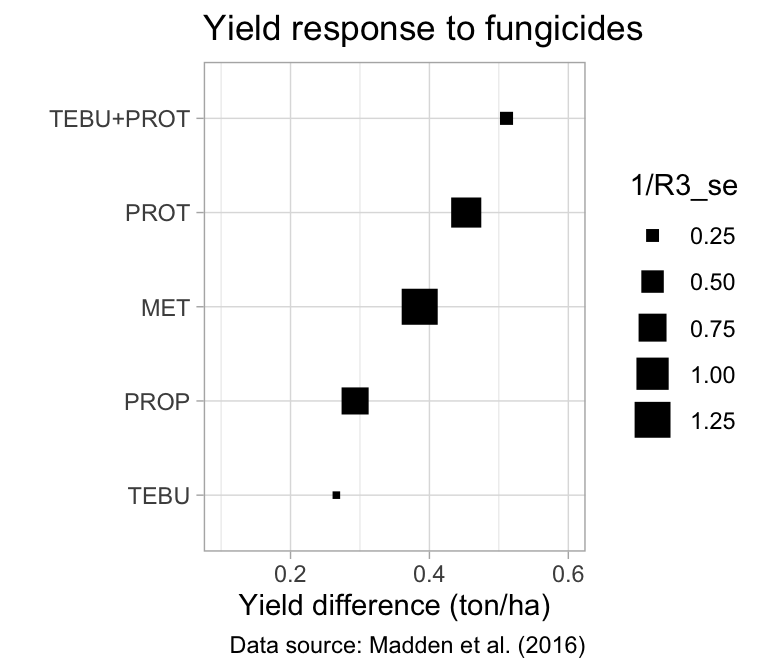

Head to head comparison

Using the best model (or any model, in fact) we can perform a head-to-head comparison based on the network model results. We can do it using {multcomp} package.

library(multcomp)
net_arm_UN_comp <-
  summary(glht(
    model = net_arm_UN,
    linfct = cbind(contrMat(rep(1, 6), type = "Tukey"))
  ))
net_arm_UN_comp

     Simultaneous Tests for General Linear Hypotheses

Fit: rma.mv(yi = yield, V = varyld, mods = ~trt, random = list(~trt | 
    factor(trial)), struct = "UN", data = wheat, method = "ML", 
    control = list(optimizer = "nlm"))

Linear Hypotheses:
            Estimate Std. Error z value Pr(>|z|)
2 - 1 == 0 -3.099135   5.288489  -0.586    0.985
3 - 1 == 0 -3.276845   6.118313  -0.536    0.990
4 - 1 == 0 -3.041372   6.338596  -0.480    0.994
5 - 1 == 0 -3.272693   4.981167  -0.657    0.976
6 - 1 == 0 -3.028717   7.240205  -0.418    0.997
3 - 2 == 0 -0.177709   1.481099  -0.120    1.000
4 - 2 == 0  0.057764   1.710301   0.034    1.000
5 - 2 == 0 -0.173558   2.367919  -0.073    1.000
6 - 2 == 0  0.070418   2.653802   0.027    1.000
4 - 3 == 0  0.235473   1.299443   0.181    1.000
5 - 3 == 0  0.004152   2.663079   0.002    1.000
6 - 3 == 0  0.248128   2.313985   0.107    1.000
5 - 4 == 0 -0.231322   2.677580  -0.086    1.000
6 - 4 == 0  0.012655   2.103377   0.006    1.000
6 - 5 == 0  0.243976   3.715404   0.066    1.000
(Adjusted p values reported -- single-step method)

We plot the results for more easily checking which differences are statistically significant (not embracing zero).

plot(net_arm_UN_comp)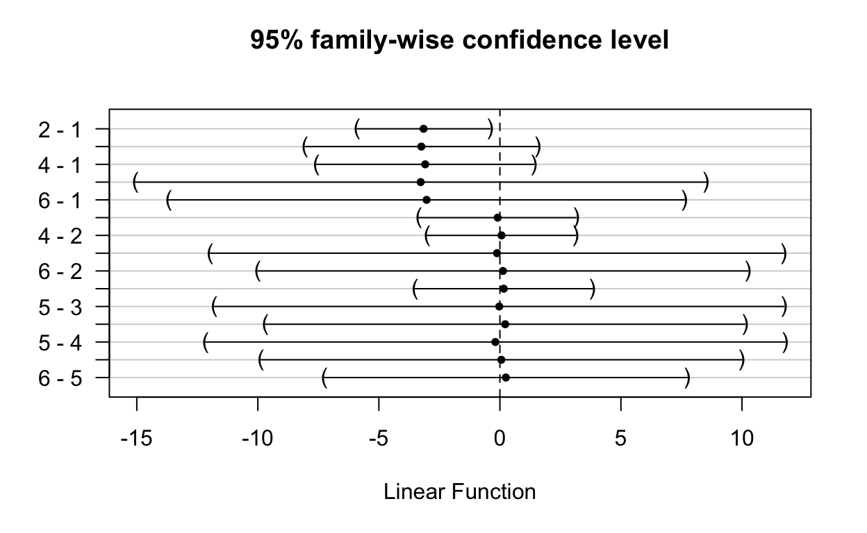

Moderator effects

In the original paper, two models were expanded to include the effect of wheat class (S = Spring wheat and W = Winter wheat) as moderator. Let’s fit the CS model as in the paper and add this moderator factor in interaction with the treatment factor. The rest is the same.

net_arm_CS_class <- rma.mv(
  yield,
  varyld,
  mods = ~ factor(trt) * class,
  method = "ML",
  random = list( ~ factor(trt) |
                   factor(trial)),
  struct = "HCS",
  data = wheat
)

As usual, we look at the model summary and check the estimates for each combination of treatment and wheat class.

summary(net_arm_CS_class)

Multivariate Meta-Analysis Model (k = 558; method: ML)

   logLik   Deviance        AIC        BIC       AICc   
-268.1385  1679.3915   574.2770   656.4398   575.6897   

Variance Components:

outer factor: factor(trial) (nlvls = 136)
inner factor: factor(trt)   (nlvls = 6)

            estim    sqrt  k.lvl  fixed      level 
tau^2.1    1.4653  1.2105    136     no       CTRL 
tau^2.2    1.2939  1.1375     86     no        MET 
tau^2.3    1.3777  1.1738     57     no       PROP 
tau^2.4    1.3796  1.1746     56     no       PROT 
tau^2.5    1.3820  1.1756    136     no       TEBU 
tau^2.6    1.3500  1.1619     87     no  TEBU+PROT 
rho        0.9834                    no            

Test for Residual Heterogeneity:
QE(df = 546) = 45668.0682, p-val < .0001

Test of Moderators (coefficients 2:12):
QM(df = 11) = 337.5307, p-val < .0001

Model Results:

                             estimate      se     zval    pval 
intrcpt                        3.0217  0.1598  18.9068  <.0001 
factor(trt)MET                 0.5226  0.0431  12.1350  <.0001 
factor(trt)PROP                0.2647  0.0499   5.3060  <.0001 
factor(trt)PROT                0.4986  0.0573   8.7051  <.0001 
factor(trt)TEBU                0.3353  0.0368   9.1056  <.0001 
factor(trt)TEBU+PROT           0.4886  0.0438  11.1556  <.0001 
classW                         0.9057  0.2114   4.2849  <.0001 
factor(trt)MET:classW         -0.1686  0.0614  -2.7444  0.0061 
factor(trt)PROP:classW        -0.1331  0.0714  -1.8648  0.0622 
factor(trt)PROT:classW        -0.1286  0.0738  -1.7437  0.0812 
factor(trt)TEBU:classW        -0.1230  0.0512  -2.4017  0.0163 
factor(trt)TEBU+PROT:classW   -0.1092  0.0606  -1.8020  0.0715 
                               ci.lb    ci.ub      
intrcpt                       2.7085   3.3350  *** 
factor(trt)MET                0.4382   0.6070  *** 
factor(trt)PROP               0.1669   0.3624  *** 
factor(trt)PROT               0.3864   0.6109  *** 
factor(trt)TEBU               0.2631   0.4075  *** 
factor(trt)TEBU+PROT          0.4028   0.5745  *** 
classW                        0.4914   1.3200  *** 
factor(trt)MET:classW        -0.2890  -0.0482   ** 
factor(trt)PROP:classW       -0.2729   0.0068    . 
factor(trt)PROT:classW       -0.2732   0.0160    . 
factor(trt)TEBU:classW       -0.2234  -0.0226    * 
factor(trt)TEBU+PROT:classW  -0.2280   0.0096    . 

---
Signif. codes:  0 '***' 0.001 '**' 0.01 '*' 0.05 '.' 0.1 ' ' 1

We can check whether the full model with the moderator is a better fit than the reduced (without moderator) model. The P-value of the LRT test suggests that indeed wheat class has a strong effect on treatment effects. This agrees with the results using SAS.

anova(net_arm_CS, net_arm_CS_class)

        df      AIC      BIC     AICc    logLik     LRT   pval 
Full    19 574.2770 656.4398 575.6897 -268.1385                
Reduced  8 583.0105 617.6054 583.2728 -283.5052 30.7335 0.0012 
                QE 
Full    45668.0682 
Reduced 55024.7841 

Wrapping up

We fitted three network models to the means of wheat yields under the effect of fungicide treatments. These models have different variance-covariance matrix. Results of these three models and, of the one expanded to include the effect of wheat class, are not identical to those obtained in Madden et al. (2016), but they are all very similar.

Useful links and other papers

• Research compendia: All the codes are made available and anyone should be able to reproduce it after downloading the research compendium and installing all the required packages (RStudio will tell you when you open the Rmd file!). You may want to check these repositories of code and data from work published in my lab using these methods: Barro et al. (2021), Barro et al. (2020), Machado et al. (2017)

• Other papers using network models (Yellareddygari et al. 2019), (Edwards Molina et al. 2018), (Paul et al. 2018), (Paul et al. 2008)

• Fitting arm-based meta-analysis with {metafor}