Introduction
The incidence and severity of plant diseases are dependent on environmental effects which is emphasised by the disease triangle (Francl 2001). Arguably the effect of temperature on disease can be the most important of environmental influences. One problem with evaluating the effect of temperatures on disease incidence and severity is the difference between air temperatures measured at a weather station and the micro-environment of the plant canopy.
When modelling plant disease outbreaks, being able to accurately estimate the conditions which lead to localised plant disease epidemics can be very useful. This led me to the R package {tealeaves} (Muir 2019), which provides functions for calculating leaf temperatures from ambient environmental inputs.
If you have not already, install the packages {tealeaves} and {nasapower} with install.packages(c("tealeaves", "nasapower")).
{tealeaves} 
library(tealeaves)Before I begin, it is worth noting {tealeaves} uses the package, units, to format the inputs and outputs (Pebesma et al. 2016). Detail about the package {tealeaves} and it’s functions can be found in Muir’s publication (Muir 2020), and in the vignettes which can be obtained by running the following commands in R:
vignette("tealeaves-introduction"),vignette("tealeaves-intermediate")
For brevity, I will not go in depth into {tealeaves} but provide a simple example using default parameters, then how to change default environmental parameters with ones obtained from the {nasapower} package.
First, a brief {tealeaves} example
lf_par <- make_leafpar()
env_par <- make_enviropar()
const <- make_constants()

Tm_leaf <-
  tleaf(leaf_par = lf_par,
        enviro_par = env_par,
        constants = const)

Tm_leaf[, c("T_leaf", "E")]
T_leaf E
1 301.4181 [K] 0.00794791 [mol/m^2/s]The function tleaf() calculates leaf temperature and evapotranspiration by solving an energy budget equation from incoming solar radiation, air temperatures, reflectance, and heat loss to wind and evapotranspiration for a leaf with certain characteristics (Muir 2019).
This equation requires these parameter inputs which describe this energy budget for calculating leaf temperature.
The parameters are created or altered through the package functions:
make_leafpar()defines the leaf parameters and characteristics,make_enviropar()sets environmental parameters,make_constants()defines the constants used in thetleaf()equation.
The tleaf() function returns an output containing details of the thermal energy absorbed and emitted, including an estimate of evapotranspiration ("E"), which assists in defining the estimated leaf temperature ("T_leaf"), given in Kelvin.
We can replace the default environmental parameters with values parsed from a weather station or remote sensing satellite data retrieved by using the R package {nasapower} (Sparks 2018; Sparks 2022).
{nasapower} 
Let’s download some hourly data using the {nasapower} (Sparks 2018; Sparks 2022) package.
More information on using the {nasapower} package can be found by calling the vignette vignette(nasapower).
library(nasapower)
np <- get_power(
  community = "ag",
  pars = c(
    "RH2M", # Relative humidity at 2 meters
    "T2M", # Air temperature at 2 meters
    "WS2M", # wind speed at 2 meters
    "ALLSKY_SFC_SW_DWN", # short wave downward solar radiation at the earth surface
    "ALLSKY_SFC_LW_DWN", # long wave downward solar radiation at the earth surface
    "PS", # surface pressure
    "ALLSKY_SRF_ALB" # Surface albedo
  ),
  temporal_api = "hourly",
  lonlat = c(150.88, -26.83),
  dates = c("2021-02-01", "2021-02-08")
)
In the get_power() function above, I have requested data from the NASA “POWER” project from the agricultural weather data collection ("ag").
These data contain all the energy balance inputs needed from a 0.5° grid cell at the specified latitude and longitude (latlong).
The coordinates I have used are just north of Dalby in Queensland, Australia.
Additionally, I have requested hourly data for the first week in February 2021 with the "temporal_api" argument.
npNASA/POWER CERES/MERRA2 Native Resolution Hourly Data
Dates (month/day/year): 02/01/2021 through 02/08/2021
Location: Latitude -26.83 Longitude 150.88
Elevation from MERRA-2: Average for 0.5 x 0.625 degree lat/lon region = 336.69 meters
The value for missing source data that cannot be computed or is outside of the sources availability range: NA
Parameter(s):
Parameters:
RH2M MERRA-2 Relative Humidity at 2 Meters (%) ;
T2M MERRA-2 Temperature at 2 Meters (C) ;
WS2M MERRA-2 Wind Speed at 2 Meters (m/s) ;
ALLSKY_SFC_SW_DWN CERES SYN1deg All Sky Surface Shortwave Downward Irradiance (MJ/hr) ;
ALLSKY_SFC_LW_DWN CERES SYN1deg All Sky Surface Longwave Downward Irradiance (W/m^2) ;
PS MERRA-2 Surface Pressure (kPa) ;
ALLSKY_SRF_ALB CERES SYN1deg All Sky Surface Albedo (dimensionless)
# A tibble: 192 × 13
LON LAT YEAR MO DY HR RH2M T2M WS2M
<dbl> <dbl> <dbl> <dbl> <dbl> <dbl> <dbl> <dbl> <dbl>
1 151. -26.8 2021 2 1 10 39.8 30.9 3.72
2 151. -26.8 2021 2 1 11 34.1 32.6 3.51
3 151. -26.8 2021 2 1 12 30.5 33.8 3.37
4 151. -26.8 2021 2 1 13 28.3 34.5 3.39
5 151. -26.8 2021 2 1 14 27.3 34.6 3.6
6 151. -26.8 2021 2 1 15 27.7 33.8 3.9
7 151. -26.8 2021 2 1 16 29.1 32.6 4.13
8 151. -26.8 2021 2 1 17 31.9 30.9 4.08
9 151. -26.8 2021 2 1 18 38.5 28.3 3.38
10 151. -26.8 2021 2 1 19 43 26.3 4.13
# ℹ 182 more rows
# ℹ 4 more variables: ALLSKY_SFC_SW_DWN <dbl>,
# ALLSKY_SFC_LW_DWN <dbl>, PS <dbl>, ALLSKY_SRF_ALB <dbl>Estimate leaf temperatures
Next, I will characterise the environmental parameters using the np data at a single time point into the tleaf().
env_par <- make_enviropar(
  replace = list(
    P = set_units(np$PS[1], "kPa"),             # Air pressure
    r = set_units(np$ALLSKY_SRF_ALB[1]),        # Albedo
    RH = set_units(np$RH2M[1]/100),             # Relative Humidity (as a proportion)
    S_sw = set_units(np$ALLSKY_SFC_SW_DWN[1],
                     "W/m^2"),                  # Short wave radiation
    T_air = set_units(
      set_units(np$T2M[1], "DegC"),
      "K"),                                     # Air temperature, converted from Celsius to Kelvin
    wind = set_units(np$WS2M[1], "m/s")         # Wind speed
    )
)
Now I can run the tleaf() function again with the updated environmental parameters.
Tm_leaf <-
  tleaf(leaf_par = lf_par,
        enviro_par = env_par,
        constants = const)

Tm_leaf[, c("T_leaf", "E")]
T_leaf E
1 299.5096 [K] 0.006604466 [mol/m^2/s]Because the outputs are specified using the {units} package I can easily convert from Kelvin back to degrees Celsius using the set_units() function again.
set_units(Tm_leaf$T_leaf, "DegC")26.35956 [°C]Leaf temperature gradients
Imputing vectors as parameters returns leaf temperature gradients across the supplied parameter permutations and not a vector of times.
Below is an example of the permutations t_leaves() processes from a vector of environmental parameters.
This is described further in the {tealeaves} vignette.
env_par <- make_enviropar(
  replace = list(
    P = set_units(np$PS[1:2], "kPa"),
    r = set_units(np$ALLSKY_SRF_ALB[1:2]),
    RH = set_units(np$RH2M[1:2] / 100), # needs to be specified as a proportion
    S_sw = set_units(np$ALLSKY_SFC_SW_DWN[1:2], "W/m^2"),
    T_air = set_units(set_units(np$T2M[1:2], "DegC"),
                      "K"),             # convert from degrees to Kelvin
    wind = set_units(np$WS2M[1:2], "m/s")
  )
)

Tm_leaves <-
  tleaves(leaf_par = lf_par,
          enviro_par = env_par,
          constants = const)

dim(Tm_leaves)
[1] 64 25# A tibble: 6 × 2
T_leaf E
[K] [mol/m^2/s]
1 299. 0.00710
2 299. 0.00724
3 300. 0.00760
4 300. 0.00775
5 299. 0.00710
6 299. 0.00724We can see that the tleaves() function uses the multiple values specified in the environmental parameters to calculate all possible gradients.
As such 64 values are returned (\(2^6\)), permutations of the input environmental parameters.
However in this example we want leaf temperature estimates over time, not space.
Leaf temperature time-series
To obtain a time series I can use the apply() function to pass the environmental parameters to tleaf() one time point at a time.
First, I need to clean up the data a little by substituting NA albedo values generated by night-time measurements.
Here I have substituted it with the mean.
tm_leaf_list <-
  apply(np, 1, function(nasa_p) {
    env_par <- make_enviropar(
      replace = list(
        P = set_units(nasa_p["PS"], "kPa"),
        r = set_units(nasa_p["ALLSKY_SRF_ALB"]),
        RH = set_units(nasa_p["RH2M"] / 100), # needs to be specified as a proportion
        S_sw = set_units(nasa_p["ALLSKY_SFC_SW_DWN"], "W/m^2"),
        T_air = set_units(set_units(nasa_p["T2M"], "DegC"),
                          "K"),               # convert from degrees to Kelvin
        wind = set_units(nasa_p["WS2M"], "m/s")
      )
    )

    return(tleaf(
      leaf_par = lf_par,
      enviro_par = env_par,
      constants = const,
      quiet = TRUE
    ))

  })

# bind the list into a data.frame
Leaf_temperatures <-
  do.call("rbind", c(tm_leaf_list, make.row.names = FALSE))

Leaf_temperatures[1:10, c("T_leaf", "E")]
T_leaf E
1 299.5096 [K] 0.006604466 [mol/m^2/s]
2 300.3629 [K] 0.007602218 [mol/m^2/s]
3 300.9245 [K] 0.008296177 [mol/m^2/s]
4 301.2553 [K] 0.008803558 [mol/m^2/s]
5 301.3194 [K] 0.009132864 [mol/m^2/s]
6 300.9297 [K] 0.009061479 [mol/m^2/s]
7 300.2532 [K] 0.008639131 [mol/m^2/s]
8 299.0727 [K] 0.007694088 [mol/m^2/s]
9 297.1887 [K] 0.005870064 [mol/m^2/s]
10 296.0459 [K] 0.005306279 [mol/m^2/s]I can now pair up the time and air temperature data from the NASA power data with the leaf temperature data. Also, I will convert temperature in Kelvin to degrees Celsius.
Leaf_temperatures$air_temp <- np$T2M

Leaf_temperatures$times <-
  as.POSIXct(paste0(np$YEAR, "-",
                    np$MO, "-",
                    np$DY, " ",
                    np$HR, ":00:00"),
             tz = "Australia/Brisbane")
Leaf_temperatures$T_leaf <-
  set_units(Leaf_temperatures$T_leaf, "DegC")
Plotting leaf temperature
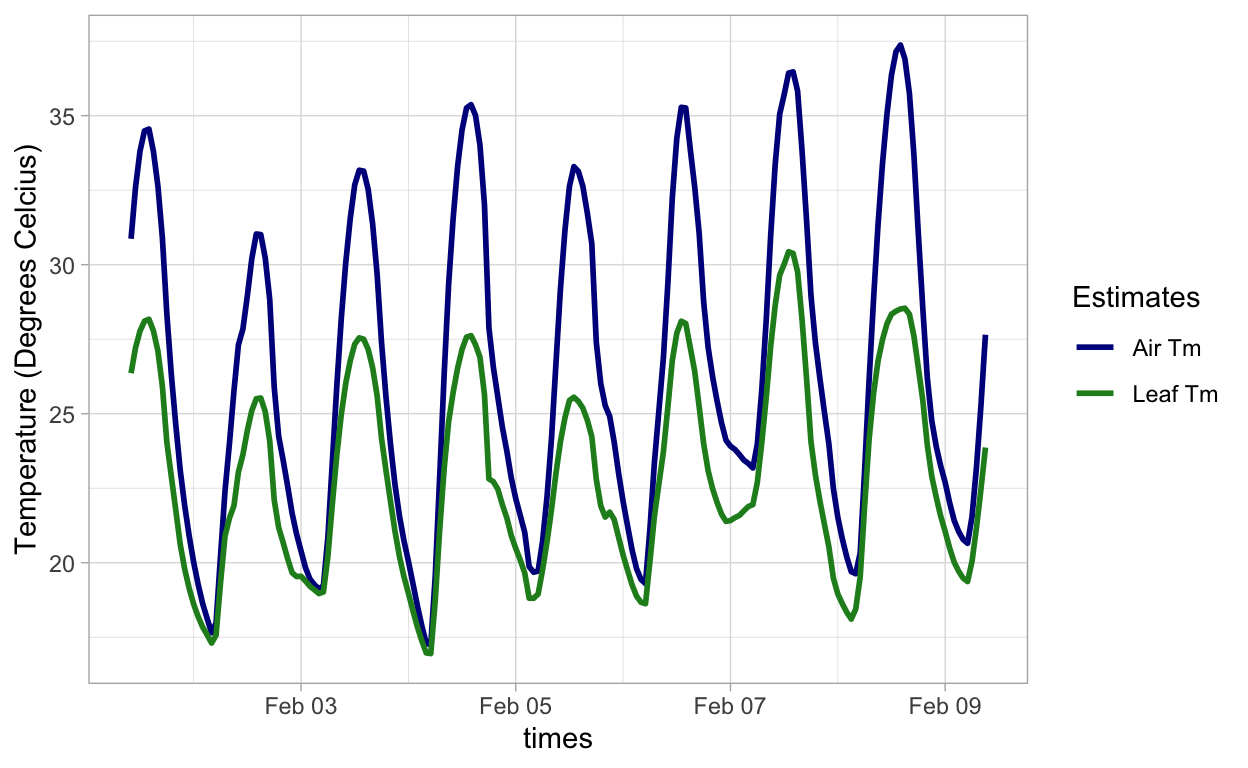
Finally, I can visualise the change in air temperature and leaf temperatures over time.
library(ggplot2)

ggplot(Leaf_temperatures,
       aes(x = times)) +
  geom_line(aes(y = air_temp, colour = "darkblue"), size = 1) +
  geom_line(aes(y = drop_units(T_leaf),
                colour = "forestgreen"), size = 1) +
  labs(y = "Temperature (Degrees Celcius)",
       color = "Estimates") +
  theme_light() +
  scale_color_manual(
    values = c("darkblue", "forestgreen"),
    labels = c("Air Tm",
               "Leaf Tm")
  )
Conclusion
Hopefully this will help get you started for using these two packages to estimate leaf and canopy temperatures. However, further parameterisation would be necessary prior to any in-depth analyses. Leaf parameters, such as leaf size, reflectance, absorbance, stomatal conductance and ratio should be carefully considered in addition to vertical environmental gradients across the height of the plant. Shading in the canopy is known to effect pathogen infection, colonisation and sporulation in addition to leaf wetness.